The Impact of a Changing Climate on the Number of Western Monarch Butterflies (Danaus plexippus) at Santa Barbara County Overwintering Sites

USDA / US Forest Service 2024

Western Monarch Butterfly

The Western monarch butterfly (Danaus plexippus) is an iconic species that was once prolific across the United States. While monarchs can be found throughout most of the US at some point during the year, the species is divided into two unofficial groups by the Continental Divide. Western monarchs are found in the western half of the United States, Eastern monarchs in the the eastern half. However, these two groups are not genetically distinct. Monarchs are a migratory species, with western monarchs spending most of the spring and summer months in Washington, Oregon, Idaho, Utah, Nevada, and Arizona. In the winter, they migrate back to Coastal California where they will spend the winter months at overwintering sites. These overwintering sites extend from Medocino County in California to Baja California in Mexico. Scientists have witnessed monarchs returning to the same overwintering sites year after year.

Overwintering Sites

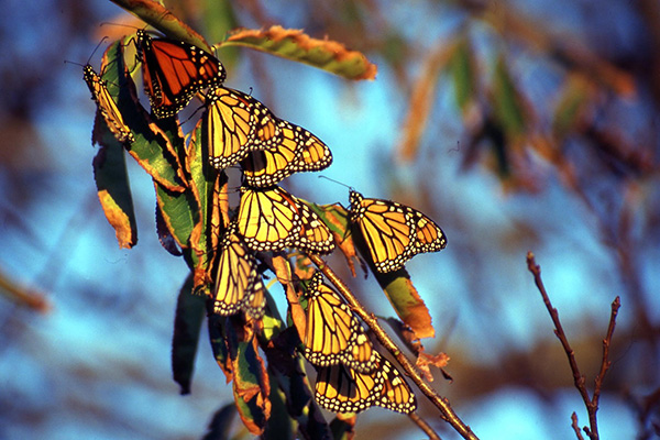
So what makes up a preferred overwintering site for monarchs? Overwintering sites typically consist of a thick grove of wind-protected trees where monarchs can cluster together and be protected from the elements. Overwintering sites are typically found to be thick groves of Eucalyptus tree species or Monterey cypress (Cupressus macrocarpa). Overwintering monarchs are particularly vulnerable to swings in temperature. Temperatures need to be sufficiently low enough that monarch metabolisims are not overworked, while not being so low that they freeze.

Import Libraries and Load Data

# Load libraries
library(tidyverse)

── Attaching core tidyverse packages ──────────────────────── tidyverse 2.0.0 ──
✔ dplyr     1.1.4     ✔ readr     2.1.5
✔ forcats   1.0.0     ✔ stringr   1.5.1
✔ ggplot2   3.5.1     ✔ tibble    3.2.1
✔ lubridate 1.9.3     ✔ tidyr     1.3.1
✔ purrr     1.0.2     
── Conflicts ────────────────────────────────────────── tidyverse_conflicts() ──
✖ dplyr::filter() masks stats::filter()
✖ dplyr::lag()    masks stats::lag()
ℹ Use the conflicted package (<http://conflicted.r-lib.org/>) to force all conflicts to become errors

library(here)

here() starts at /Users/rachelswick/Documents/MEDS/rfswick.github.io

library(kableExtra)

Attaching package: 'kableExtra'

The following object is masked from 'package:dplyr':

    group_rows

library(dynlm)

Loading required package: zoo

Attaching package: 'zoo'

The following objects are masked from 'package:base':

    as.Date, as.Date.numeric

# Load monarch data
monarch_data <- read_csv(here("blogs", "2024-monarch-count-analysis", "data", "XercesSociety_WMC_Data_3.19.2024.csv"))

New names:
Rows: 389 Columns: 40
── Column specification
──────────────────────────────────────────────────────── Delimiter: "," chr
(10): SITE NAME, COUNTY, 2016, 2017, 2018, 2019, 2020, 2021, 2022, 2023 dbl
(1): SITE ID num (27): 1997, 1998, 1999, 2000, 2001, 2002, 2003, 2004, 2005,
2006, 2007, ... lgl (2): ...39, ...40
ℹ Use `spec()` to retrieve the full column specification for this data. ℹ
Specify the column types or set `show_col_types = FALSE` to quiet this message.
• `` -> `...39`
• `` -> `...40`

# Load SB rainfall data
carp_rain <- read_csv(here("blogs", "2024-monarch-count-analysis", "data", "carpinteria-fire-station-rain-gauge.csv"))

New names:
Rows: 2953 Columns: 13
── Column specification
──────────────────────────────────────────────────────── Delimiter: "," chr
(1): code dbl (6): station id, water year, year, month, day, daily rain lgl
(6): ...8, ...9, ...10, ...11, ...12, ...13
ℹ Use `spec()` to retrieve the full column specification for this data. ℹ
Specify the column types or set `show_col_types = FALSE` to quiet this message.
• `` -> `...8`
• `` -> `...9`
• `` -> `...10`
• `` -> `...11`
• `` -> `...12`
• `` -> `...13`

mont_rain <- read_csv(here("blogs", "2024-monarch-count-analysis", "data", "cold-springs-debris-basin-rain-gauge.csv"))

New names:
• `` -> `...8`

Warning: One or more parsing issues, call `problems()` on your data frame for details,
e.g.:
  dat <- vroom(...)
  problems(dat)

Rows: 1778 Columns: 8
── Column specification ────────────────────────────────────────────────────────
Delimiter: ","
chr (1): code
dbl (6): station id, water year, year, month, day, daily rain
lgl (1): ...8

ℹ Use `spec()` to retrieve the full column specification for this data.
ℹ Specify the column types or set `show_col_types = FALSE` to quiet this message.

sb_rain <- read_csv(here("blogs", "2024-monarch-count-analysis", "data", "santa-barbara-rain-gauge.csv"))

New names:
Rows: 4708 Columns: 13
── Column specification
──────────────────────────────────────────────────────── Delimiter: "," chr
(1): code dbl (6): station id, water year, year, month, day, daily rain lgl
(6): ...8, ...9, ...10, ...11, ...12, ...13
ℹ Use `spec()` to retrieve the full column specification for this data. ℹ
Specify the column types or set `show_col_types = FALSE` to quiet this message.
• `` -> `...8`
• `` -> `...9`
• `` -> `...10`
• `` -> `...11`
• `` -> `...12`
• `` -> `...13`

lompoc_rain <- read_csv(here("blogs", "2024-monarch-count-analysis", "data", "surf-beach-rain-gauge.csv"))

New names:
• `` -> `...8`
• `` -> `...9`
• `` -> `...10`
• `` -> `...11`
• `` -> `...12`

Warning: One or more parsing issues, call `problems()` on your data frame for details,
e.g.:
  dat <- vroom(...)
  problems(dat)

Rows: 2249 Columns: 12
── Column specification ────────────────────────────────────────────────────────
Delimiter: ","
dbl (6): station id, water year, year, month, day, daily rain
lgl (6): code, ...8, ...9, ...10, ...11, ...12

ℹ Use `spec()` to retrieve the full column specification for this data.
ℹ Specify the column types or set `show_col_types = FALSE` to quiet this message.

goleta_rain <- read_csv(here("blogs", "2024-monarch-count-analysis", "data", "ucsb-rain-gauge.csv"))

Rows: 2816 Columns: 7
── Column specification ────────────────────────────────────────────────────────
Delimiter: ","
chr (1): code
dbl (6): station id, water year, year, month, day, daily rain

ℹ Use `spec()` to retrieve the full column specification for this data.
ℹ Specify the column types or set `show_col_types = FALSE` to quiet this message.

Clean Monarch Data

# Add "y_" to beginning of year columns to select columns more easily
names(monarch_data)[4:ncol(monarch_data)] <- paste0("y_", names(monarch_data)[4:ncol(monarch_data)])

# Select monarch data from Santa Barbara county
monarch_sb <- monarch_data %>% 
  filter(COUNTY == "Santa Barbara") %>% 
  mutate(across(starts_with("y_"), as.integer))

Warning: There were 6 warnings in `mutate()`.
The first warning was:
ℹ In argument: `across(starts_with("y_"), as.integer)`.
Caused by warning:
! NAs introduced by coercion
ℹ Run `dplyr::last_dplyr_warnings()` to see the 5 remaining warnings.

# Remove "y_" from the beginning of year columns
names(monarch_sb) <- gsub("^y_", "", names(monarch_sb))

# Make the year columns tidy and drop unneeded columns
monarch_sb <- monarch_sb %>% 
  pivot_longer(cols = starts_with("19") | starts_with("20"),  
               names_to = "YEAR", 
               values_to = "COUNT") %>% 
  select(-starts_with("LS"), -starts_with("..."))

Select Monarch Data

# Number of NA values at each site
monarch_sb_site <- monarch_sb %>% 
  group_by(`SITE NAME`) %>% 
  summarize(NA_Count = sum(is.na(COUNT)))

# Total monarch count by year
monarch_sb_total <- monarch_sb %>% 
  group_by(YEAR) %>% 
  summarize(Total_Count = sum(COUNT, na.rm = TRUE))

# Average monarch count by year
monarch_sb_avg_1 <- monarch_sb %>% 
  group_by(YEAR) %>% 
  summarize(Avg_Count = round(mean(COUNT, na.rm = TRUE), 0)) %>% 
  rename(year = YEAR,
         avg_count = Avg_Count)

# Average monarch count by year
monarch_sb_avg <- monarch_sb %>% 
  group_by(YEAR) %>% 
  summarize(Avg_Count = round(mean(COUNT, na.rm = TRUE), 0)) %>% 
  rename(year = YEAR,
         avg_count = Avg_Count)

# Elwood Mesa average monarch count by year
monarch_ellwood_avg <- monarch_sb %>% 
  filter(str_starts(`SITE NAME`, "Ellwood"))  %>% 
  group_by(YEAR) %>% 
  summarize(Avg_Count = round(mean(COUNT, na.rm = TRUE), 0))

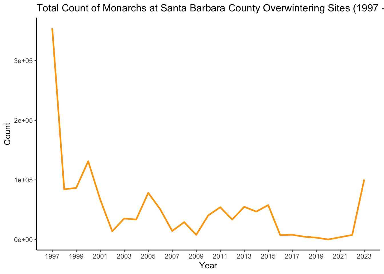
Monarch Count Trends

# Update year to be a date object
monarch_sb_total$YEAR <- as.Date(paste(monarch_sb_total$YEAR, "01", "01", sep = "-"))

# Plot
ggplot(data = monarch_sb_total, aes(x = YEAR, y = Total_Count, group = 1)) +
  geom_line(color = "orange",
            lwd = 1) +
  labs(title = "Total Count of Monarchs at Santa Barbara County Overwintering Sites (1997 - 2023)",
       x = "Year",
       y = "Count") +
  scale_x_date(breaks = "2 years", labels = scales::date_format("%Y")) +
  theme_classic()

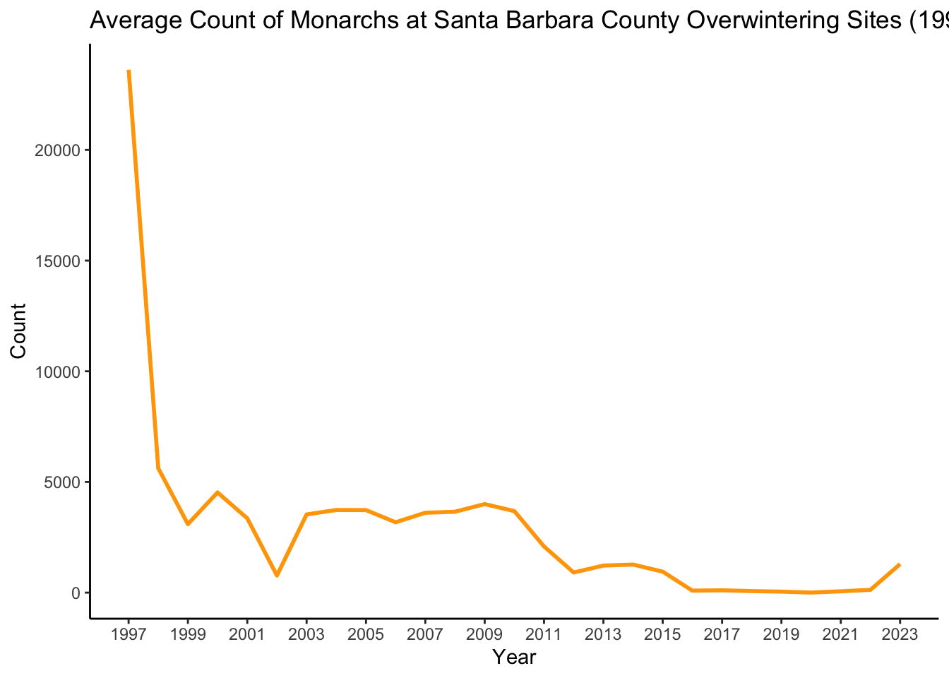
# Update year to be a date object
monarch_sb_avg_1$year <- as.Date(paste(monarch_sb_avg_1$year, "01", "01", sep = "-"))

# Plot
ggplot(data = monarch_sb_avg_1, aes(x = year, y = avg_count, group = 1)) +
  geom_line(color = "orange",
            lwd = 1) +
  labs(title = "Average Count of Monarchs at Santa Barbara County Overwintering Sites (1997 - 2023)",
       x = "Year",
       y = "Count") +
  scale_x_date(breaks = "2 years", labels = scales::date_format("%Y")) +
  theme_classic()

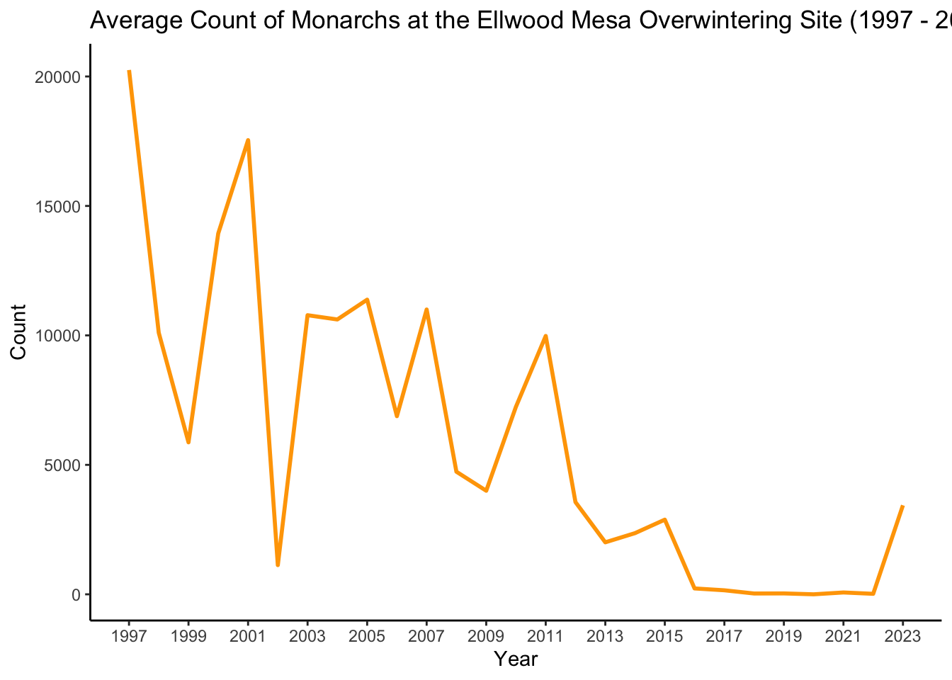
# Update year to be a date object
monarch_ellwood_avg$YEAR <- as.Date(paste(monarch_ellwood_avg$YEAR, "01", "01", sep = "-"))

# Plot
ggplot(data = monarch_ellwood_avg, aes(x = YEAR, y = Avg_Count, group = 1)) +
  geom_line(color = "orange",
            lwd = 1) +
  labs(title = "Average Count of Monarchs at the Ellwood Mesa Overwintering Site (1997 - 2023)",
       x = "Year",
       y = "Count") +
  scale_x_date(breaks = "2 years", labels = scales::date_format("%Y")) +
  theme_classic()

Santa Barbara County Rainfall Data

# UCSB rain gauge data
goleta_rain_dec <- goleta_rain %>% 
  filter(month == 12) %>% 
  rename("daily_rain" = "daily rain")

# Cold Springs Debris Basin rain gauge
mont_rain_dec <- mont_rain %>% 
  filter(month == 12) %>% 
  rename("daily_rain" = "daily rain")

# Carpinteria Fire Station rain gauge data
carp_rain_dec <- carp_rain %>% 
  filter(month == 12) %>% 
  rename("daily_rain" = "daily rain")

# Santa Barbara rain gauge data
sb_rain_dec <- sb_rain %>% 
  filter(month == 12) %>% 
  rename("daily_rain" = "daily rain")

# Surf Beach rain gauge data
lompoc_rain_dec <- lompoc_rain %>% 
  filter(month == 12) %>% 
  rename("daily_rain" = "daily rain")

ggplot(data = goleta_rain_dec, aes(x = daily_rain)) +
  geom_histogram(color = "grey",
                 fill = "lightblue",
                 bins = 40) +
  labs(title = "Rainfall at UCSB Rain Gauge in December (1951 - 2024)",
       x = "Daily Rainfall (Inches)",
       y = "Count") +
  theme_bw()

ggplot(data = mont_rain_dec, aes(x = daily_rain)) +
  geom_histogram(color = "grey",
                 fill = "lightblue",
                 bins = 40) +
  labs(title = "Rainfall at Cold Springs Debris Basin Rain Gauge in December (1964 - 2024)",
       x = "Daily Rainfall (Inches)",
       y = "Count") +
  theme_bw()

Determine rain events occurring in the 80th percentile or above

# Find 80th percentile of daily rain data
upper_bound_g <- quantile(goleta_rain_dec$daily_rain, 0.80, na.rm = TRUE)

# Identify values outside 90% of the average
goleta_rain_dec$outside_range <- goleta_rain_dec$daily_rain > upper_bound_g

goleta_rain_grouped <- goleta_rain_dec %>% 
  select(-code) %>% 
  group_by(year) %>% 
  summarize(rain_events = sum(outside_range == TRUE)) %>% 
  mutate(rain_gauge = "UCSB")

# Find 80th percentile of daily rain data
upper_bound_m <- quantile(mont_rain_dec$daily_rain, 0.80, na.rm = TRUE)

# Identify values outside 90% of the average
mont_rain_dec$outside_range <- mont_rain_dec$daily_rain > upper_bound_m

mont_rain_grouped <- mont_rain_dec %>% 
  select(-code) %>% 
  group_by(year) %>% 
  summarize(rain_events = sum(outside_range == TRUE)) %>% 
   mutate(rain_gauge = "Cold Springs")

# Find 80th percentile of daily rain data
upper_bound_c <- quantile(carp_rain_dec$daily_rain, 0.80, na.rm = TRUE)

# Identify values outside 90% of the average
carp_rain_dec$outside_range <- carp_rain_dec$daily_rain > upper_bound_c

carp_rain_grouped <- carp_rain_dec %>% 
  select(-code) %>% 
  group_by(year) %>% 
  summarize(rain_events = sum(outside_range == TRUE)) %>% 
   mutate(rain_gauge = "Carp Fire Station")

# Find 80th percentile of daily rain data
upper_bound_s <- quantile(sb_rain_dec$daily_rain, 0.80, na.rm = TRUE)

# Identify values outside 90% of the average
sb_rain_dec$outside_range <- sb_rain_dec$daily_rain > upper_bound_s

sb_rain_grouped <- sb_rain_dec %>% 
  select(-code) %>% 
  group_by(year) %>% 
  summarize(rain_events = sum(outside_range == TRUE)) %>% 
  mutate(rain_gauge = "Santa Barbara")

# Find 80th percentile of daily rain data
upper_bound_l <- quantile(lompoc_rain_dec$daily_rain, 0.80, na.rm = TRUE)

# Identify values outside 90% of the average
lompoc_rain_dec$outside_range <- lompoc_rain_dec$daily_rain > upper_bound_l

lompoc_rain_grouped <- lompoc_rain_dec %>% 
  select(-code) %>% 
  group_by(year) %>% 
  summarize(rain_events = sum(outside_range == TRUE)) %>% 
  mutate(rain_gauge = "Surf Beach")

# Combine rain gauge data together
rain_gauge_data <- bind_rows(mont_rain_grouped, goleta_rain_grouped, carp_rain_grouped, sb_rain_grouped, lompoc_rain_grouped)

# Average number of storm events across all rain gauges
storm_events <- rain_gauge_data %>% 
  group_by(year) %>% 
  summarize(avg_storm_events = round(mean(rain_events), 2))

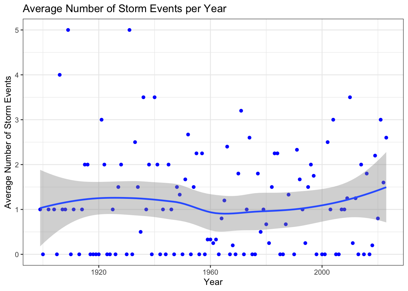
Determine if the number of storm events has been increasing over time

ggplot(storm_events, aes(x = year, y = avg_storm_events)) +
  geom_point(color = "blue") +
  geom_smooth() +
  labs(title = "Average Number of Storm Events per Year",
       x = "Year",
       y = "Average Number of Storm Events") +
  theme_bw()

`geom_smooth()` using method = 'loess' and formula = 'y ~ x'

# Determine if there is correlation between time and storm events
cor(storm_events$avg_storm_events, storm_events$year)

[1] -0.008362463

Look at Maximum Rain Events

# UCSB rain gauge data
goleta_rain_max <- goleta_rain %>% 
  filter(month == 12) %>% 
  rename("daily_rain" = "daily rain") %>% 
  group_by(year) %>% 
  summarise(max_storm = max(daily_rain)) %>% 
  mutate(rain_gauge = "UCSB")

# Cold Springs Debris Basin rain gauge
mont_rain_max <- mont_rain %>% 
  filter(month == 12) %>% 
  rename("daily_rain" = "daily rain") %>% 
  group_by(year) %>% 
  summarise(max_storm = max(daily_rain)) %>% 
  mutate(rain_gauge = "Cold Springs")

# Carpinteria Fire Station rain gauge data
carp_rain_max <- carp_rain %>% 
  filter(month == 12) %>% 
  rename("daily_rain" = "daily rain") %>% 
  group_by(year) %>% 
  summarise(max_storm = max(daily_rain)) %>% 
  mutate(rain_gauge = "Carp Fire Station")

# Santa Barbara rain gauge data
sb_rain_max <- sb_rain %>% 
  filter(month == 12) %>% 
  rename("daily_rain" = "daily rain") %>% 
  group_by(year) %>% 
  summarise(max_storm = max(daily_rain)) %>% 
  mutate(rain_gauge = "Santa Barbara")

# Surf Beach rain gauge data
lompoc_rain_max <- lompoc_rain %>% 
  filter(month == 12) %>% 
  rename("daily_rain" = "daily rain") %>% 
  group_by(year) %>% 
  summarise(max_storm = max(daily_rain)) %>% 
  mutate(rain_gauge = "Surf Beach")

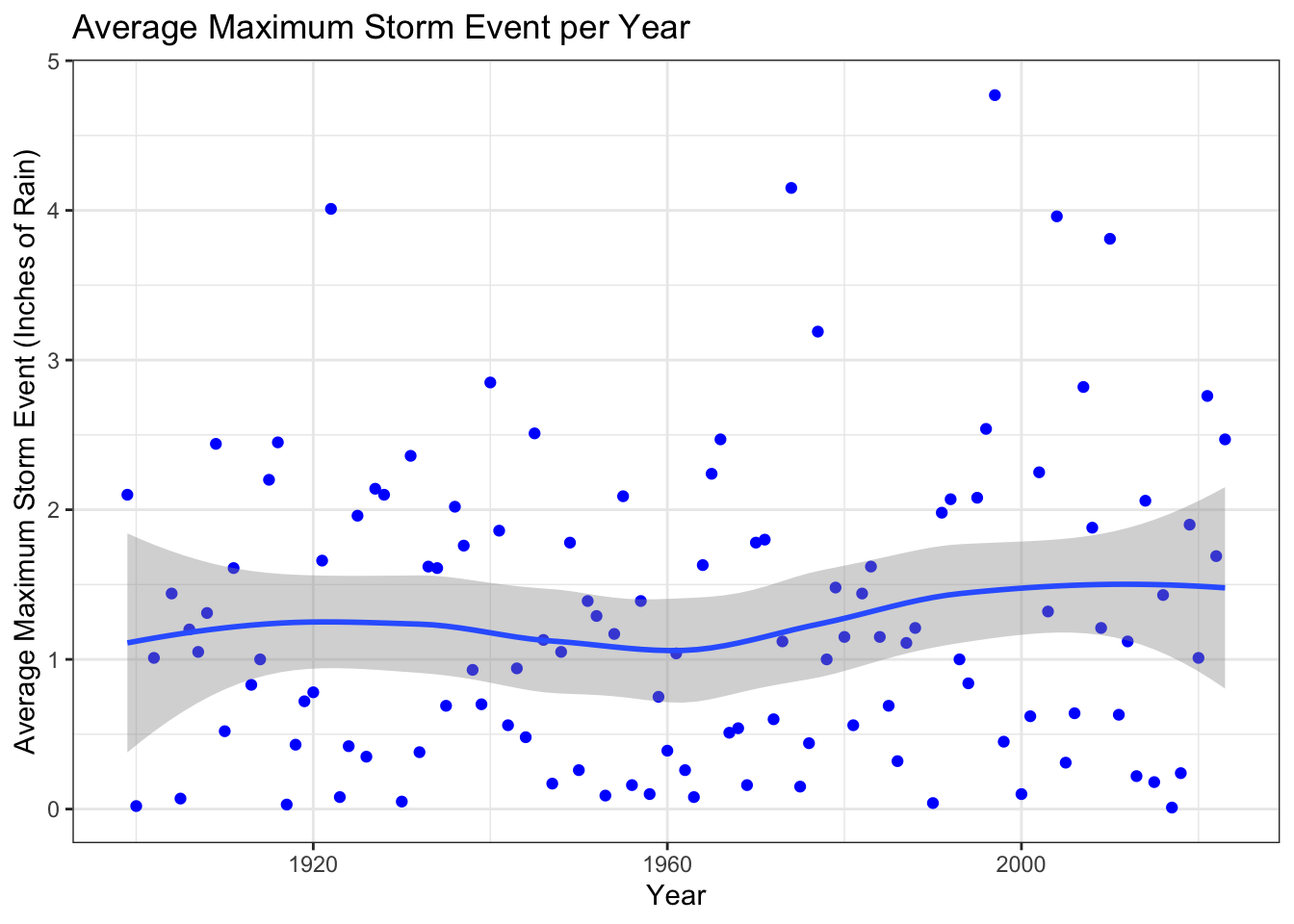
# Combine rain gauge data together
rain_gauge_max <- bind_rows(mont_rain_max, goleta_rain_max, carp_rain_max, sb_rain_max, lompoc_rain_max)

# Average number of storm events across all rain gauges
max_storm_events <- rain_gauge_max %>% 
  group_by(year) %>% 
  summarize(max_storm_event = round(mean(max_storm), 2)) 

ggplot(max_storm_events, aes(x = year, y = max_storm_event)) +
  geom_point(color = "blue") +
  geom_smooth() +
  labs(title = "Average Maximum Storm Event per Year",
       x = "Year",
       y = "Average Maximum Storm Event (Inches of Rain)") +
  theme_bw()

`geom_smooth()` using method = 'loess' and formula = 'y ~ x'

# Determine if there is correlation between time and storm events
cor(max_storm_events$max_storm_event, max_storm_events$year)

[1] 0.1005336

Combine rain and monarch data together

# Combine rain and monarch data
monarch_rain_df <- merge(monarch_sb_avg, max_storm_events, by = "year")
monarch_rain_df <- merge(monarch_rain_df, storm_events, by = "year")

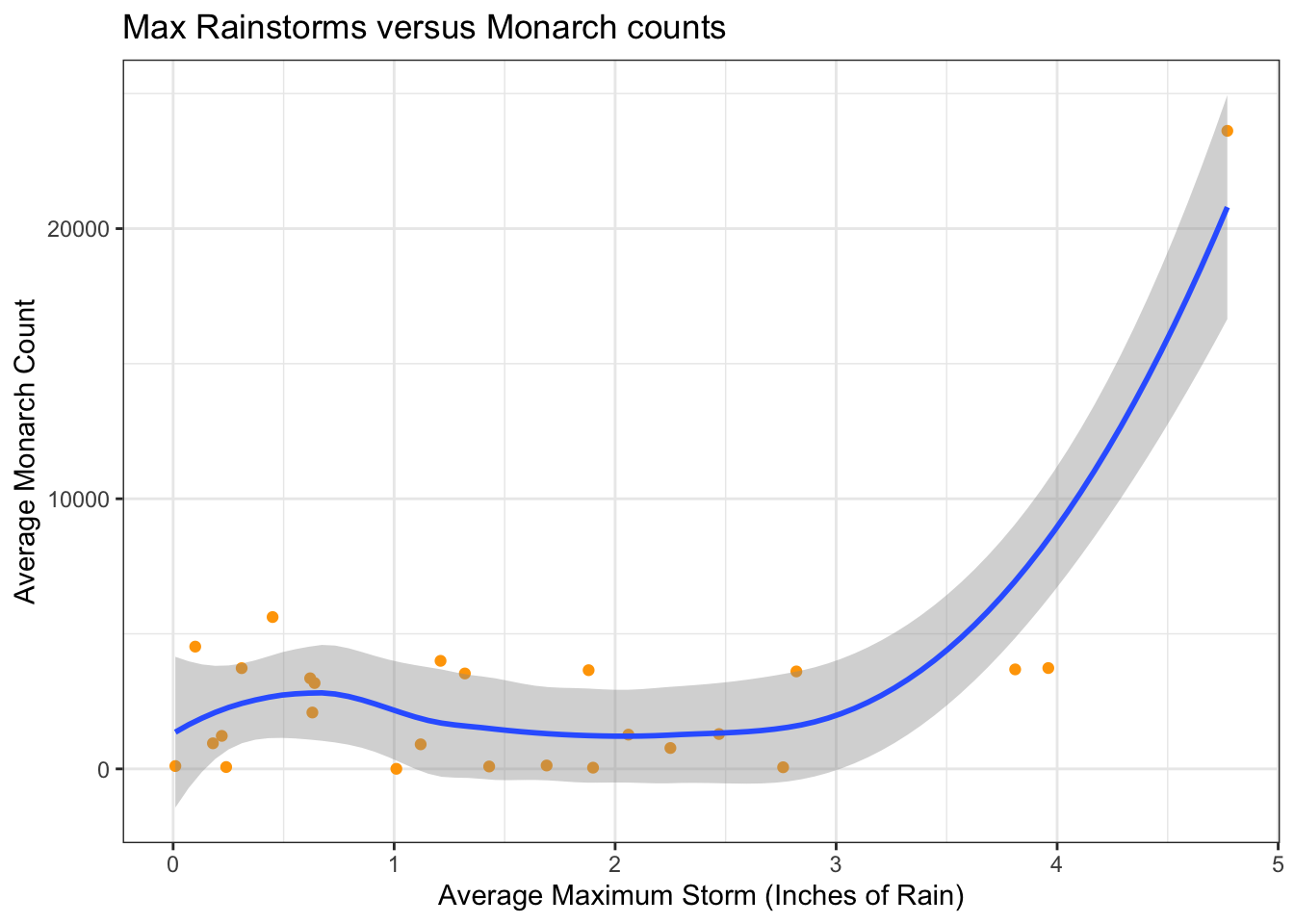
ggplot(monarch_rain_df, aes(x = max_storm_event, y = avg_count)) +
  geom_point(color = "orange") +
  geom_smooth() +
  labs(title = "Max Rainstorms versus Monarch counts",
       x = "Average Maximum Storm (Inches of Rain)",
       y = "Average Monarch Count") +
  theme_bw()

`geom_smooth()` using method = 'loess' and formula = 'y ~ x'

# Determine if there is correlation between time and storm events
cor(monarch_rain_df$max_storm_event, monarch_rain_df$avg_count)

[1] 0.4857452

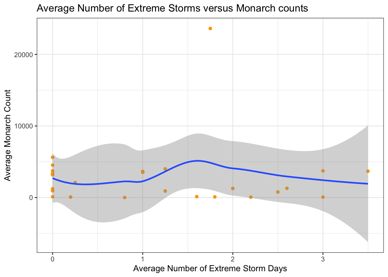
ggplot(monarch_rain_df, aes(x = avg_storm_events, y = avg_count)) +
  geom_point(color = "orange") +
  geom_smooth() +
  labs(title = "Average Number of Extreme Storms versus Monarch counts",
       x = "Average Number of Extreme Storm Days",
       y = "Average Monarch Count") +
  theme_bw()

`geom_smooth()` using method = 'loess' and formula = 'y ~ x'

# Determine if there is correlation between time and average number of storm events
cor(monarch_rain_df$avg_storm_events, monarch_rain_df$avg_count)

[1] 0.01968187

lm(monarch_rain_df$avg_count ~ monarch_rain_df$max_storm_event)

Call:
lm(formula = monarch_rain_df$avg_count ~ monarch_rain_df$max_storm_event)

Coefficients:
                    (Intercept)  monarch_rain_df$max_storm_event  
                          269.2                           1711.8  

summary(lm(monarch_rain_df$avg_count ~ monarch_rain_df$avg_storm_events))

Call:
lm(formula = monarch_rain_df$avg_count ~ monarch_rain_df$avg_storm_events)

Residuals:
    Min      1Q  Median      3Q     Max 
-2979.0 -2577.1 -1154.6   720.2 20681.0 

Coefficients:
                                 Estimate Std. Error t value Pr(>|t|)  
(Intercept)                       2799.07    1339.39   2.090   0.0474 *
monarch_rain_df$avg_storm_events    79.97     829.24   0.096   0.9240  
---
Signif. codes:  0 '***' 0.001 '**' 0.01 '*' 0.05 '.' 0.1 ' ' 1

Residual standard error: 4660 on 24 degrees of freedom
Multiple R-squared:  0.0003874, Adjusted R-squared:  -0.04126 
F-statistic: 0.009301 on 1 and 24 DF,  p-value: 0.924

acf(monarch_rain_df$avg_count, main = "Autocorrelation Function of Time Series")

ols_mod <- lm(avg_count ~ max_storm_event, monarch_rain_df)
summary(ols_mod)

Call:
lm(formula = avg_count ~ max_storm_event, data = monarch_rain_df)

Residuals:
    Min      1Q  Median      3Q     Max 
-4933.7 -2934.1  -396.2  1495.5 15185.6 

Coefficients:
                Estimate Std. Error t value Pr(>|t|)  
(Intercept)        269.2     1252.1   0.215   0.8316  
max_storm_event   1711.8      628.8   2.722   0.0119 *
---
Signif. codes:  0 '***' 0.001 '**' 0.01 '*' 0.05 '.' 0.1 ' ' 1

Residual standard error: 4074 on 24 degrees of freedom
Multiple R-squared:  0.2359,    Adjusted R-squared:  0.2041 
F-statistic: 7.411 on 1 and 24 DF,  p-value: 0.01188

residual_acf <- acf(resid(ols_mod), plot = FALSE)
tibble(Lag = residual_acf$lag, ACF = as.vector(residual_acf$acf)) %>% 
  ggplot(aes(Lag, ACF)) +
  geom_line(lwd = 2) +
  geom_hline(yintercept = 0,
             linetype = "dashed",
             color = "orange",
             linewidth = 1.5) +
  theme_bw() +
  labs(title = "Lag model")

adl_mod <- dynlm(
  avg_count ~ L(avg_count, 1) + max_storm_event,
  ts(monarch_rain_df, start = 1996)
)
summary(adl_mod)

Time series regression with "ts" data:
Start = 1997, End = 2021

Call:
dynlm(formula = avg_count ~ L(avg_count, 1) + max_storm_event, 
    data = ts(monarch_rain_df, start = 1996))

Residuals:
   Min     1Q Median     3Q    Max 
 -1684  -1203   -268   1083   2063 

Coefficients:
                 Estimate Std. Error t value Pr(>|t|)    
(Intercept)     965.99032  484.06376   1.996 0.058508 .  
L(avg_count, 1)   0.26405    0.05918   4.462 0.000195 ***
max_storm_event 226.18797  241.72431   0.936 0.359572    
---
Signif. codes:  0 '***' 0.001 '**' 0.01 '*' 0.05 '.' 0.1 ' ' 1

Residual standard error: 1333 on 22 degrees of freedom
Multiple R-squared:  0.4761,    Adjusted R-squared:  0.4284 
F-statistic: 9.995 on 2 and 22 DF,  p-value: 0.0008166

adl_resid_acf <- acf(resid(adl_mod), plot = FALSE)
tibble(Lag = adl_resid_acf$lag, ACF = as.vector(adl_resid_acf$acf)) %>% 
  ggplot(aes(Lag, ACF)) +
  geom_hline(yintercept = 0,
             linetype = "dashed",
             color = "orange",
             lwd = 1.5) +
  geom_line(lwd = 2) +
  theme_bw() +
  labs(title = "Autoregressive Distrubted Lag Model")